Key facts
The Sentinel per-fastener defect detection model operates at above 95% accuracy on the Deutsche Bahn deployment — measured against ground-truth labels validated by DB's senior inspection teams across hundreds of thousands of frames.
Source · Dronehub × Deutsche Bahn deployment validation metrics
Rail-fastener defect taxonomy at the operator-grade level spans roughly 15-25 distinct defect classes — loose bolts, missing fasteners, plate damage, weld condition, sleeper-tie pattern anomalies, ballast displacement, drainage features, and the long-tail of rare but operationally-critical defects.
Source · Rail-inspection per-asset taxonomy literature; Deutsche Bahn inspection categorisation
Training-data discipline — labels generated by Deutsche Bahn's own senior inspection teams rather than crowdsourced annotators — produced the largest single accuracy gain in the per-fastener detector's development.
Source · Sentinel model-development methodology
3 more key facts
Synthetic data — physics-based defect simulation augmented onto base rail imagery — closes the gap on rare-but-critical defect classes (e.g. specific failure modes that are operationally important but statistically infrequent in the field archive).
Source · Sentinel training-pipeline architecture
False-positive rate matters more than false-negative rate at the operator-workflow level — a high false-positive rate floods the maintenance planner with non-actionable detections and erodes operator trust; the per-fastener detector is tuned for high precision before recall, with severity scoring providing the recall-side coverage.
Source · Operator-workflow analysis for rail-inspection AI
Per-fastener accuracy continues improving on-deployment — the model retrains continuously against operator feedback (false positives confirmed by ground-truth inspection, missed defects identified during scheduled maintenance), with model versions deployed to production on a structured release cadence.
Source · Sentinel on-deployment retraining architecture
In this piece
The 95%+ per-fastener defect detection accuracy at Deutsche Bahn scale is the single most-cited number in the Sentinel architecture story. It's also the number that gets the most surface-level treatment. This post is the technical companion to the Deutsche Bahn case study — what the 95%+ measurement actually means, how it was achieved, where the next accuracy gain comes from, and what the procurement-grade workflow implications are.
If you're evaluating Sentinel for licensing, building a partnership around a new rail-operator deployment, or just trying to understand what "AI rail inspection at 95%+ accuracy" really means — this is the briefing.
What "per-fastener" actually means
Most AI inspection narratives talk about detection rates at the network or asset-class level. Sentinel measures at the per-fastener level, and the distinction matters.
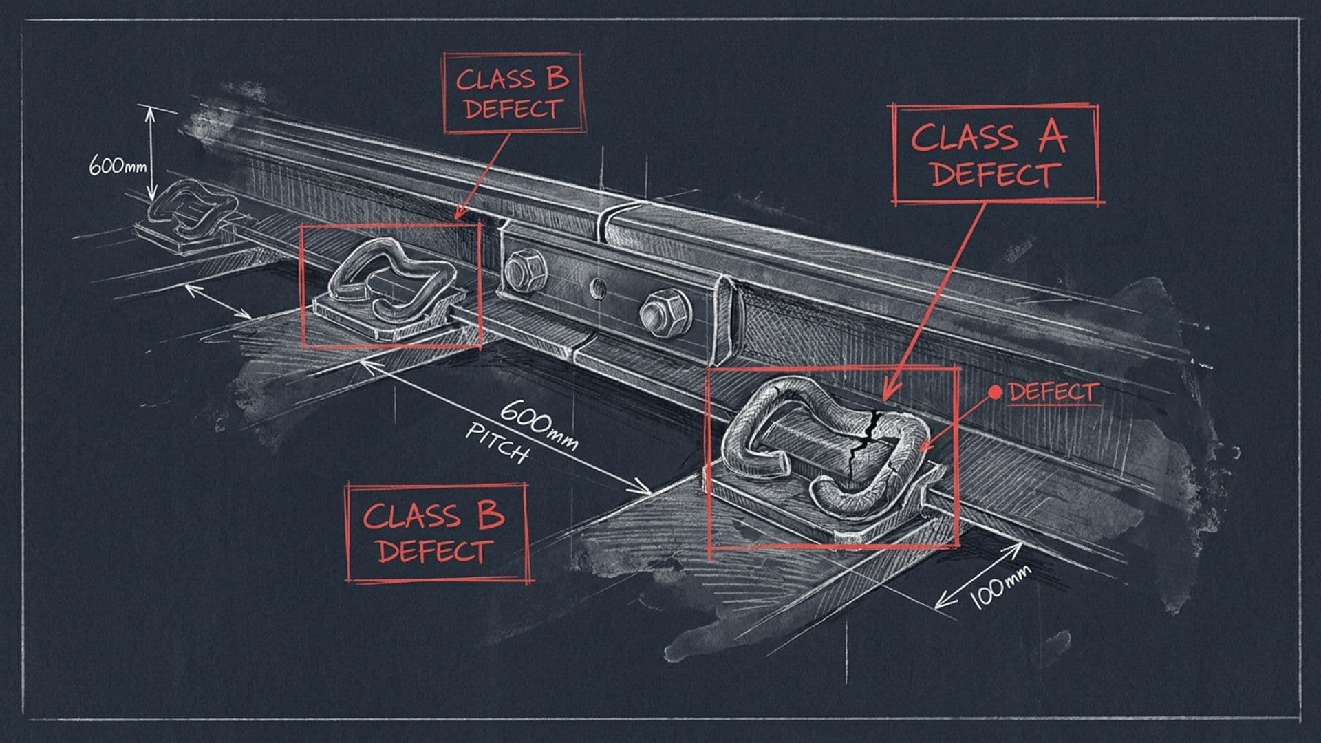
A drone captures imagery during inspection — typically 30-60 frames per second of high-resolution rail-bed imagery, gigabytes per inspection run. The fasteners — bolts, clip fittings, plate hardware that hold the rail to its sleepers — appear in every frame. A continuous section of track has fasteners every 60 to 80 centimetres; a kilometre of track has roughly 15,000 fasteners visible across the captured imagery.
Per-fastener defect detection is the discrete classification decision on each of those individual fasteners. The model identifies each fastener's position in the frame, classifies its condition state across the trained defect taxonomy, severity-scores the detection, and pins the result to GPS coordinates plus rail-segment identifiers. The 95%+ accuracy measurement is on the per-fastener classification decision — does the model correctly identify each fastener's condition state against ground-truth labels assigned by Deutsche Bahn's senior inspection teams.
The measurement is not "does the AI find some defect somewhere in the inspection run" (a much easier problem — a competent vision model gets >99% on that). It's "does the AI correctly classify each individual fastener" at the unit level. The denominator is the total fastener count; the numerator is the count of fasteners correctly classified including condition state, severity score, and defect-class assignment.
Across hundreds of thousands of frames in the Deutsche Bahn deployment, the model's per-fastener classification accuracy validates above 95% against ground-truth inspector labels. That's the headline number.
The defect taxonomy
Per-fastener classification operates against a defect taxonomy with roughly 15-25 distinct classes depending on how granularly the operator wants to discriminate. The major categories at Deutsche Bahn:
Loose bolts. Torque-loss indicators on bolted fittings. Visible signs include slight rotation from the installed position, subtle tilt of the bolt head, paint-line displacement (where a torque-indicator paint mark crosses the bolt-plate boundary), and pattern deviations across adjacent bolts in the same fitting group. The model classifies loose bolts at multiple severity levels — early-stage torque drift, mid-stage torque loss, late-stage near-failure.
Missing fasteners. The most operationally critical category — direct safety implication. The model identifies the expected fastener position and classifies whether the fastener is present, partially present (e.g., broken), or absent. A missing fastener detection routes to the maintenance planner with the highest priority severity score.
Plate damage. Cracking, deformation, or displacement of the rail-foot plate that holds the rail to the sleeper. Plate damage is operationally important because it affects load distribution and can accelerate adjacent fastener failure. The model classifies plate damage across multiple types — surface cracking, structural deformation, displacement-from-design-position, weld-zone damage where the plate joins adjacent components.
Weld condition. Visible weld defects in the rail itself (rail-to-rail welds between segments) or in welded fittings. Weld classification is technically challenging because weld defects have subtle visual signatures and high variance in appearance; the per-asset taxonomy specialisation matters here.
Sleeper-tie anomalies. Rotation, displacement, or decay of the rail sleepers. Wood-sleeper degradation patterns differ from concrete-sleeper degradation patterns; the model handles both with separate sub-classifications.
Ballast displacement. Sub-track ballast condition that affects fastener-plate seating. Ballast displacement is detected from the drone's downward-look imagery; the model classifies displacement extent and pattern.
Drainage features. Drainage condition along the track corridor, which affects long-term track stability. Less time-critical than direct-fastener defects but operationally relevant for the maintenance-planning cadence.
Long-tail categories. A long tail of operationally-rare classes — specific failure modes that develop in narrow conditions, regional anomalies that affect particular sections of the network, defect patterns that the operator's regulator has flagged for specific reporting requirements.
Each operator can extend or restrict the taxonomy based on their network's specific asset profile and the regulator's reporting requirements. The taxonomy is a configuration of the model federation, not a hardcoded part of the architecture.
The training-data discipline that moved the ceiling
The accuracy ceiling for a per-fastener detector is bounded by training data quality more than by model architecture. Across the first deployment phases on Deutsche Bahn, the team experimented with model architecture changes — transformer variants, depth-vs-width tradeoffs, training-loss strategies — and none moved the ceiling more than 2-3 percentage points. What moved the ceiling by 10-15 percentage points at a time was training-data discipline.
Three properties of training data matter most.
Labeller authority. Labels generated by Deutsche Bahn's senior inspection teams produce models that outperform models trained against crowdsourced annotations by a wide margin. The reason is judgement encoding. A senior inspector labelling a fastener as "loose-trending-torque-loss" combines visible evidence (slight rotation, subtle tilt, paint-line displacement) with experience-based context (typical degradation patterns for this fastener type in this network's conditions). The label carries the inspector's encoded knowledge. A crowdsourced annotator labelling the same fastener as "fastener-present" or "fastener-defective" applies a much coarser judgement that loses the inspector's domain expertise. Across many fasteners, the accuracy delta between senior-inspector labels and crowdsourced labels runs 10-15+ percentage points. That's the gain we got from labeller authority.
Per-asset taxonomy specialisation. A single "rail defect" classifier trained on the full asset taxonomy underperforms a federation of per-defect-class specialised detectors. The fastener detector trains on labelled fastener imagery. The plate-damage detector trains on labelled plate-damage imagery. The weld-condition detector trains on labelled weld imagery. Each detector is specialised against a narrower distribution and a more disciplined taxonomy. The combined system outperforms the unified model on every cross-validation fold.
Synthetic supplementation for rare classes. Some defects are operationally critical but statistically infrequent in the field archive. Specific failure modes that develop in narrow conditions, regional anomalies, or defect patterns the operator's preventive maintenance had historically prevented from manifesting at scale. The model needs training examples to learn these patterns, but the field archive doesn't have enough. Synthetic data — physics-based defect simulation augmented onto base rail imagery — closes the rare-class gap. We model the defect's visual signature physically (how the surface would look under that failure mode, accounting for the optical properties of the materials involved) and overlay it onto real captured imagery, producing labelled examples the model can train against. The synthetic data is supplemental to real data, not a replacement.
The combined effect of these three properties produces the 95%+ accuracy at deployment scale. Training-data discipline first, taxonomy specialisation second, architecture last.
The false-positive economy
The 95%+ accuracy number is necessary but not sufficient at the operator-workflow level. The maintenance planner's experience of the detector depends on the precision-recall tradeoff more than on aggregate accuracy.
A high false-positive rate floods the planner with non-actionable detections. The planner reviews each one, finds it's not a real defect, dismisses it, moves on. After a few cycles of this, operator trust in the AI erodes. The planner starts ignoring detections wholesale, or treating them as a checkbox exercise rather than as actionable inputs. The detector's value to the workflow collapses.
A high false-negative rate has the inverse failure — the planner misses real defects because the AI didn't surface them. But for the rail-inspection use case specifically, missed defects are partly compensated by the regular re-inspection cadence (drones run inspection on every rail segment at scheduled intervals, so a missed defect on one pass typically surfaces on the next). False positives don't compensate; each one consumes the planner's review attention permanently.
The per-fastener detector is therefore tuned for high precision before recall. The decision threshold for surfacing a detection to the planner is set at a confidence level that produces a low false-positive rate; the recall-side coverage comes from severity scoring. A high-confidence detection surfaces at high severity. A lower-confidence detection at high severity also surfaces (the planner wants to know about a likely-real critical defect even at lower confidence). A lower-confidence detection at low severity drops below the actionable threshold but stays in the audit trail.
The combined output is high-precision actionable detections plus a separate audit-trail layer for the lower-confidence detections. The planner's workflow is protected from false-positive overload while the lower-confidence detections remain available for upstream investigation when needed.
On-deployment continuous retraining
The accuracy ceiling moves up over the first 6-18 months of deployment as the training data deepens. The continuous retraining cycle handles three input sources:
Operator feedback on detections. When the planner reviews a detection and finds it's a false positive (no actual defect on ground-truth inspection), that's a high-value training signal — a hard negative that the model failed to discriminate. When the planner finds a real defect that the AI missed (typically identified during scheduled maintenance crew inspection), that's a hard positive the model needs to learn. Both feed back into the next training cycle.
Ambiguous cases resolved by senior inspectors. Detections at the boundary of the confidence threshold sometimes route to senior-inspector review. The inspector's resolution decision becomes a high-value training example for the model's hard categories — the ones where the boundary between classes is genuinely ambiguous and the model needs the inspector's judgement to learn.
Structured retraining cycles. The training data accumulates continuously, but model retraining runs on a structured release cadence — typically every 4-8 weeks depending on the operator's change-management process. Each retraining cycle produces a new model version that improves against the accumulated training data, gets validated against held-out cross-validation sets, and deploys to production after change-management sign-off.
The dominant source of continuous improvement is the operator-feedback loop. The first deployment ships with the model trained against the labelled field archive plus synthetic supplementation. The first 12-18 months of on-deployment retraining adds operator-validated labels at a rate that materially deepens the training data. By month 24 of deployment, the per-fastener detector approaches the per-asset accuracy ceiling that's been validated at the Deutsche Bahn-class deployments.
What this means for new operators
For a rail operator evaluating Sentinel deployment — the 95%+ per-fastener accuracy is what the deployment converges to over 12-24 months, not what ships on day one. The initial deployment ships at operationally-useful accuracy (high enough to be a meaningful improvement over manual track-walking inspection) and improves continuously through the operator-feedback loop. The procurement question is therefore not "does the AI ship at 95% on day one" but "does the deployment architecture support the continuous-improvement path to that accuracy ceiling."
For a non-rail operator evaluating Sentinel for a different asset class (wind blades, pipeline welds, transmission towers, port quay walls) — the per-fastener architecture is reusable. The defect taxonomy changes (per-blade defects, per-weld defects, per-tower defects), the training data sources change (the operator's existing inspection archive plus appropriate synthetic supplementation), but the labeller-authority discipline, the per-asset taxonomy specialisation, and the false-positive-aware precision-recall tradeoff all transfer.
For a regulator evaluating AI-driven inspection across an operator pool — the per-fastener measurement is the right granularity for procurement-grade audit. It measures the operationally-meaningful decision (does the AI correctly classify each individual asset) rather than the aggregate-level "does the AI find some defects somewhere" question. Regulators that want to verify AI-driven inspection performance can request per-fastener accuracy metrics against an independent ground-truth panel.
The Sentinel architecture deep-dive is at /blog/halo-cloud-architecture-deep-dive. The Deutsche Bahn deployment case study is at /projects/deutsche-bahn. The AI rail inspection at national scale narrative is at /blog/ai-rail-inspection-national-scale-deutsche-bahn. The rail industry context is at /industries/rail. For a deployment conversation, open the contact form.
FAQ
- What does 'per-fastener defect detection' actually measure?
- Discrete classification on individual rail fasteners — bolts, clip fittings, plate hardware — in captured drone imagery. The model identifies each fastener in the frame, classifies its condition state across the trained defect taxonomy, severity-scores the detection, and pins the result to GPS coordinates plus rail-segment identifiers. The 95%+ accuracy measurement is on the per-fastener classification decision — does the model correctly identify each fastener's condition state against ground-truth labels assigned by senior inspectors. The measurement is not 'does the AI find some defect somewhere' (a much easier problem); it's 'does the AI correctly classify each individual fastener' at the unit level.
- What's the actual defect taxonomy?
- Roughly 15-25 distinct defect classes depending on how granularly the operator wants to discriminate. The major categories include: loose bolts (torque-loss indicators on bolted fittings), missing fasteners (the most operationally critical category — direct safety implication), plate damage (cracking, deformation, displacement of the rail-foot plate), weld condition (visible weld defects, weld-zone degradation, weld-line cracking), sleeper-tie anomalies (rotation, displacement, decay), ballast displacement (sub-track ballast condition that affects fastener-plate seating), and a long tail of operationally-rare categories. Each operator can extend or restrict the taxonomy based on their network's specific asset profile and the regulator's reporting requirements.
- Why did labeller authority matter so much?
- Because inspection judgement is encoded in the label. A senior inspector labelling a fastener as 'loose-trending-torque-loss' is making a judgement call that combines visible-evidence (slight rotation, subtle tilt, paint-line displacement) with experience-based context (typical degradation pattern for this fastener type in this network's conditions). A crowdsourced annotator labelling the same fastener as 'fastener-present' or 'fastener-defective' applies a much coarser judgement that loses the inspector's encoded knowledge. The model trained against senior-inspector labels learned the inspector's judgement; the model trained against crowdsourced labels learned a coarser classification. Across many such fasteners, the accuracy difference between the two label sources runs 10-15+ percentage points. That's the gain we got from labeller authority.
- How does synthetic data help?
- By closing the gap on rare-but-critical defect classes. Some defects are operationally critical but statistically rare in the field archive — for example, specific failure modes that develop in narrow conditions or that the network has historically prevented through other inspection cadences. The model needs training examples to learn these patterns, but the field archive doesn't contain enough. Synthetic data is physics-based defect simulation augmented onto base rail imagery — we model the defect's visual signature physically and overlay it onto real captured imagery, producing labelled examples that the model can train against. The synthetic data is not a replacement for real data; it's a supplement for the rare-class tail.
- What's the false-positive vs false-negative tradeoff?
- At the operator-workflow level, false-positive rate matters more than false-negative rate. A high false-positive rate floods the maintenance planner with non-actionable detections — the planner has to review each detection, find it's not a real defect, dismiss it, and move on. After a few cycles of this, operator trust in the AI erodes and the planner starts ignoring detections wholesale. The per-fastener detector is tuned for high precision before recall, with severity scoring providing the recall-side coverage. A 'maybe' detection at high severity surfaces to the planner; a 'maybe' detection at low severity drops below the actionable threshold. The combined output is high-precision actionable detections plus a separate audit-trail layer for the lower-confidence detections.
- Where does the next accuracy gain come from?
- Three directions. First, deeper training data — as the deployment runs, the model gathers new labels from operator feedback. The training data deepens; the accuracy ceiling moves up. This is the dominant source of continuous improvement. Second, taxonomy refinement — adding new defect classes for operationally-relevant patterns that the initial taxonomy didn't separately classify. Third, cross-operator pattern learning — when Sentinel deploys across multiple rail operators, the model learns from the combined operator pool while keeping per-operator data sovereign by architecture. The federation effect raises the model's capability on rare classes without breaking operator-data isolation.